RIdeogram Tutorial
You are a bright-eyed student who has a new genome assembly in hand and wanted to create cool new graphs for publications.
Jumping into the deep end of work can be fun but also a bit annoying as you are trying to wrap your head of getting to the end product.
As a self-taught bioinformatician, I'm trying to write this guide for past me and to other newbies a la Learning in Public.
I hope you have some Unix Skills that you don't get warned about.
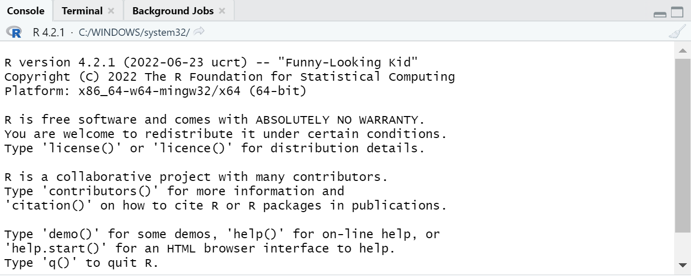
What is R?
R is a coding language typically used by biologists for it's friendly syntax and well developed packages that can make publishable science figures.
I love R because it is free and open source! It is a language for statistics analysis with relatively little coding when compared to Python.
It is a command line based code, so one line at a time. Don't use just Base R.
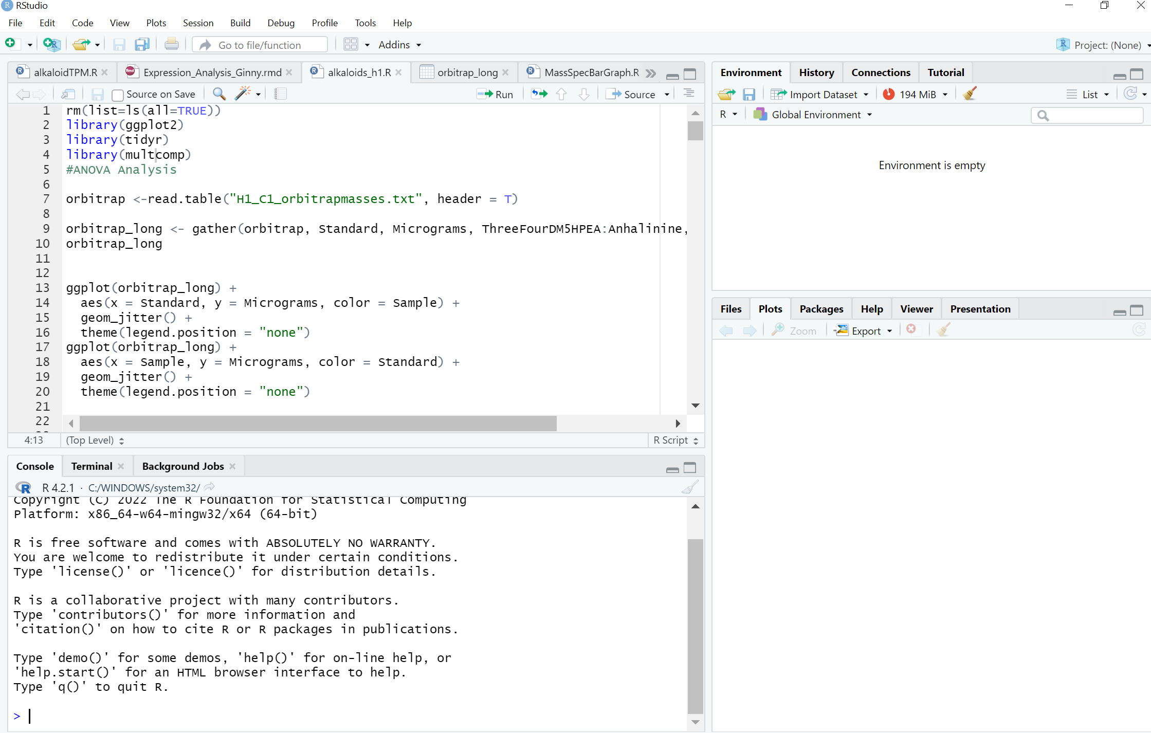
What is RStudio?
Instead, go for an environment that allows to you code, plot, and manage your work at the same time. You can see that RStudio is split into 4 panels, a coding panel in the top left, a list of active objects in the top right, the command line console in the bottom left, and the file/plots/help in the bottom right.
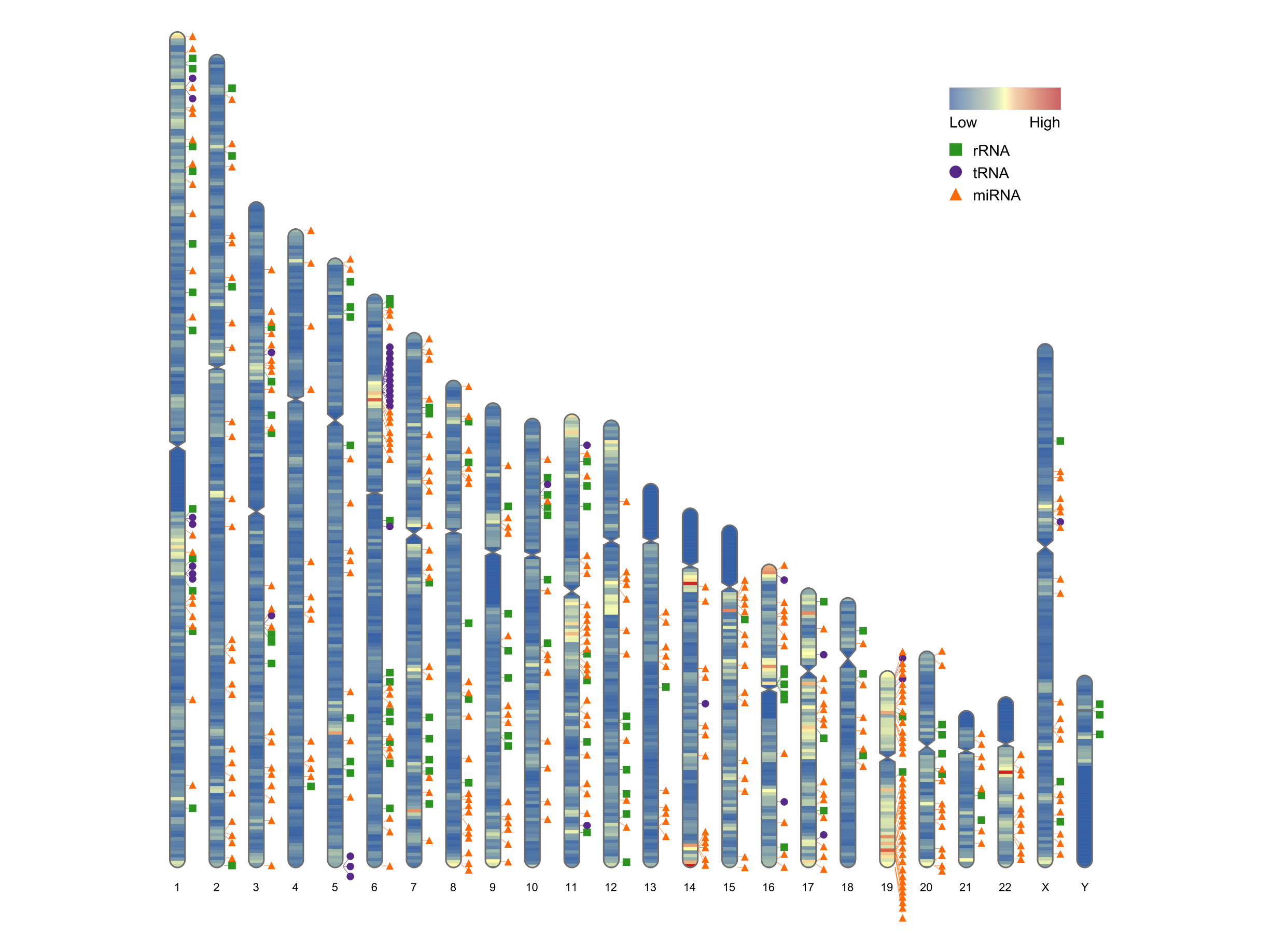
What is RIdeogram?
An ideogram is a line up of all the chromosomes in the genome side by side.
Set Up
First, it may be smart to set up version control and projects. I didn't do this at the start and I regret it as I updated my code and things broke out of the blue.
File > New Project > Pick a Place to store your project and off you go!
It should retain the current version of everything in that project.
We need to install the packages now which are little bundles of code that we can use for our projects thanks to the open source developers.
I would like to preface that one of the developers of RIdeogram has a vignette here: https://cran.r-project.org/web/packages/RIdeogram/vignettes/RIdeogram.html - the images and base code used in this tutorial are from this vignette.
In any case, this is about wrangling the how do we get the necessary files?
Install the packages:
install.packages("RIdeogram")
Activate the Packages:
require(RIdeogram)
The three data files you need are a karyotype, gene density, and gene annotations.
karyotype_set <- read.table("karyotype.txt", sep = "\t", header = T, stringsAsFactors = F)
gene_density <- read.table("data_1.txt", sep = "\t", header = T, stringsAsFactors = F)
Random_RNAs_500 <- read.table("data_2.txt", sep = "\t", header = T, stringsAsFactors = F)
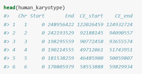
Karyotype
The first hurdle, where are you going to get the karyotype for your special model organism?
It has the chromosome number, start, end, and optionally, centromere start and end. It is not required if you don't know where they are.
I hope you are reading this as someone who already has a UNIX installation. You'll have to do some tinkering if you don't with *** . I hope you do, otherwise, where are you doing that genome analysis?
Download Samtools with their simple commands
https://github.com/samtools/samtools?tab=readme-ov-file
Then run the faidx command to get chromosome length information
samtools faidx /<path to genome>/genome.fa > output.fai
Use the code less to view the contents of the output
less outout.fai
This will get you the end coordinates. I created my karyotype in Excel for easy editing. The ideogram will generate based on the order you enter, it will not rearrange itself. Copy this file to the project directory.
Gene Density
The format of the file gave me the hint. A gff3 file is a standard file format and can be generated with alignment programs.
I personally used gmap: http://research-pub.gene.com/gmap/
Navigate to a directory where you can install programs. Copy the link of one of the version files and use
#Download the program
wget http://research-pub.gene.com/gmap/src/gmap-gsnap-2025-04-18.tar.gz

#unzip the program in its own folder
tar -xzvf gmap-gsnap-2025-04-18.tar.gz

#You may need to edit the configure file
#Compiling the program
    ./configure
    make
    make check   (optional)
    make install
Generate the gff3 file with gmap.
gmap –D <genome location> –d <genome database> –f gff3_gene –-ordered
Copy the gff3 file to the directory and load it into the environment. The feature can be gene, mRNA, exon, whatever the columns are available.
gene_density <- GFFex(input = "genome.gff3", karyotype = "karyotype.txt", feature = "gene", window = 1000000)
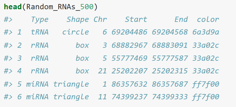
Gene Annotations
If you wanted to have certain annotations on the ideogram, it can be generated any way you want.
I personally blasted the genome for my specific locations because there were so few of them and labelled them with their gene names under the "Type" column. The color column are hex codes.
I'm a fan of coolors to generate hex codes. https://coolors.co/
However, if your gmap query was well annotated, simply use those coordinates.
Finally, run them all together with this code.
ideogram(karyotype = karyotype_set, overlaid = gene_density, label = Random_RNAs_500, label_type = "marker")

convertSVG("chromosome.svg", device = "png")
It is telling the program to look at these chromosomes, then add colours for gene density in the overlay, and label the ideogram with the list from Random_RNAs_500.